We had a guest lecture from Sid Sen on computational complexity and algorithm analysis.
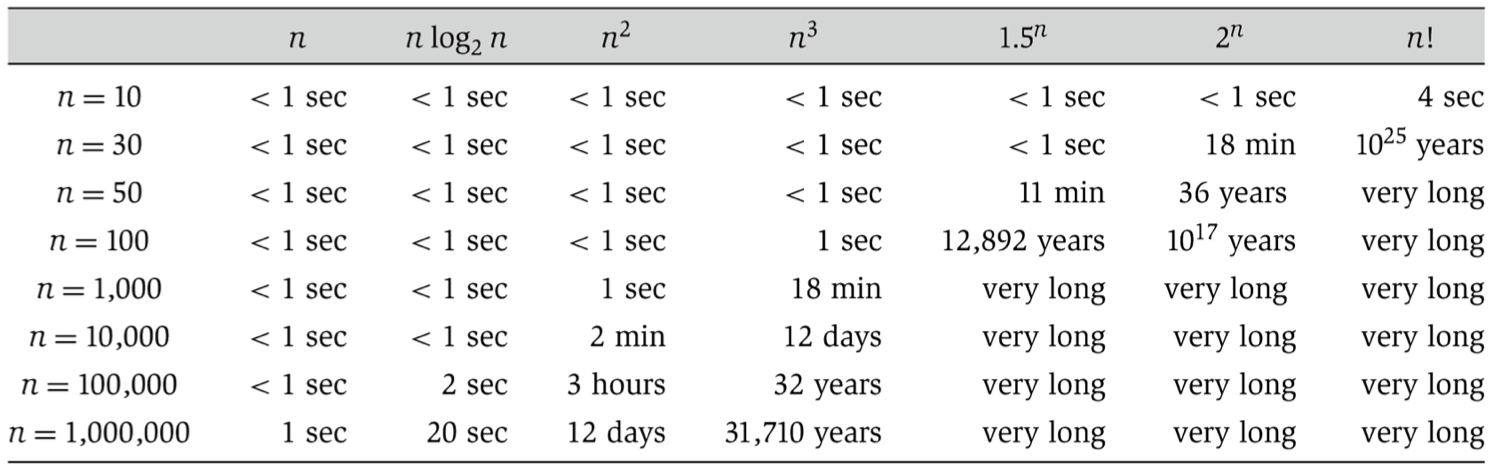
Sid discussed various ways of analyzing how long algorithms take to run, focusing on worst-case analysis. We discussed asymptotic notation (big-O for upper bounds, big-omega for lower bounds, and big-theta for tight bounds). The table above, from Algorithm Design by Kleinberg and Tardos, shows how long we should expect different algorithms to run on modern hardware. The key takeaway is that knowing how to match the right algorithm to your dataset is important. For instance, when you’re dealing with millions of observations, only linear (or maybe linearithmic) time algorithms are practical.
A few other references:
- A beginner’s guide to big-O notation
- Another introduction to big-O
- The big-O cheatsheet
We touched upon a few more advanced topics around the tradeoff between how long something takes to run and how much space it requires. Sid gave a brief overview of skip lists and mentioned some more recent work by his advisor, Robert Tarjan, on zip trees (video lecture here).
Sid finished his lecture by discussing how this applies to something as simple as taking the intersection of two lists, useful for joining different tables.
A naive approach of comparing all pairs of elements takes quadratic time.
It’s relatively easy to do much better by sorting and merging the two sets, reducing this to n log(n) time.
And if we’re willing to trade space for time, we can use a hash table to get the job done in linear time, known as a hash join.
We used the end of lecture to revisit the command line and finish up a few leftover topics. See last week’s post for links to code from class.
Next week we’ll discuss data manipulation in R. In preparation, make sure to set up R and the tidyverse packages. If you’re new to R, in addition to the readings in R4DS book, check out the CodeSchool and DataCamp intro to R courses. Also have a look at the slides and code we’ll discuss in class next week, which are up on github.